Normality Test in SciTrack: How to Use It and Interpret the Results

Before choosing a statistical test, you need to know whether your numeric variable is approximately normally distributed. SciTrack now includes a built-in Normality Test inside your project analytics tools. This guide shows you exactly how to use it and how to interpret the results so you can confidently choose parametric or non-parametric analysis.

Related guides that pair well with this tool: How to Choose Outcomes and Define Endpoints, How to Critically Appraise a Study.

What the normality test answers (and what it does not)

A normality test helps you decide whether a variable is close enough to a normal distribution to justify certain methods (for example, t-tests, ANOVA, linear regression assumptions, and parametric confidence intervals). It does not prove that data are perfectly normal. It gives evidence about whether the deviation from normality is statistically detectable.

Important: Normality is most critical for residuals in many models, but in practical applied research, checking the distribution of your main continuous variables is a helpful first step.

How to open the Normality Test tool in SciTrack

1. Open your project.
2. Go to Analytics or Analysis Tools.
3. Select Normality Test.

Step-by-step: running a normality test

Step 1: Choose your data source

Depending on how SciTrack is configured in your project, you may either:

• Select a dataset already stored in the project (recommended), or
• Paste values manually, or
• Upload a CSV/Excel file (if enabled).

Step 2: Select the variable (column) to test

Choose the numeric column you want to evaluate (for example, age, BMI, lab values, ICU length of stay). If you have a grouping variable (like male vs female or intervention vs control), select it only if the tool supports group-wise normality checks.

Step 3: Choose the test(s)

SciTrack may provide one or more tests. Use these practical rules:

• Shapiro–Wilk: excellent default for small to moderate sample sizes.
• Kolmogorov–Smirnov (with Lilliefors correction): commonly used, often less powerful than Shapiro–Wilk.
• Anderson–Darling: gives more weight to tail behavior (useful if tails matter).

If SciTrack offers only one test, that is fine. The most important part is combining the p-value with visual plots (histogram and Q–Q plot).

Step 4: Run the analysis

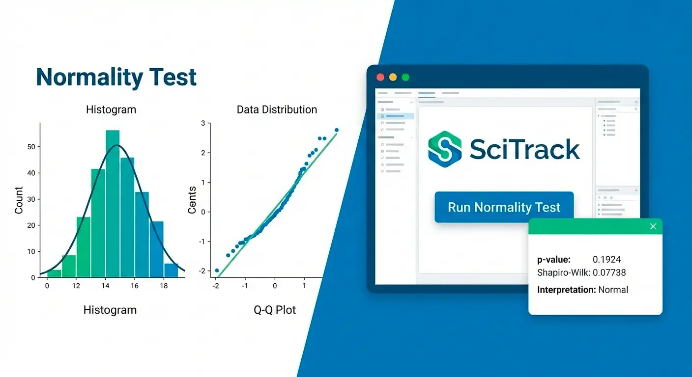
Click Run (or the equivalent action button). SciTrack will compute the statistics and show results panels and plots.

How to interpret the results

1) The p-value (what it means)

In most normality tests, the null hypothesis is: the data are normally distributed. If p < 0.05, the test suggests a statistically detectable deviation from normality.

However, p-values are sensitive to sample size:

• Small samples: you may fail to detect non-normality even if the distribution is not normal.
• Large samples: tiny, unimportant deviations can produce very small p-values.

Practical rule: interpret the p-value together with the plots and the clinical meaning of the variable.

2) Histogram (shape check)

A histogram helps you see skewness, outliers, and whether there is a single bell-shaped mode. Mild skewness may still be acceptable depending on your planned test and sample size.

3) Q–Q plot (the fastest visual test)

In a Q–Q plot, points should fall roughly along a straight line if the data are approximately normal. Systematic curves indicate skewness. Strong deviations at the ends suggest heavy tails or outliers.

What to do next: choosing the right statistical test

Once you know the distribution, you can decide the next step:

• Looks approximately normal (or large n with mild deviations): consider parametric tests (t-test, ANOVA) and report mean ± SD.
• Clearly non-normal / skewed: consider non-parametric tests (Mann–Whitney, Kruskal–Wallis) and report median (IQR).
• Outliers dominate: check data quality, consider robust methods, transformations, or sensitivity analyses.

If you choose transformations (log, square root), document the reason and interpret results carefully in the original scale when possible.

Common mistakes (and how to avoid them)

• Relying only on p-value: always check histogram and Q–Q plot.
• Testing normality after choosing the analysis: plan your approach in advance if possible.
• Ignoring groups: if you compare groups, check distribution within each group (if feasible).
• Confusing normality of data vs normality of residuals: for regression models, residual diagnostics matter most.

FAQ

What is the best normality test?

There is no single best test for every scenario. Shapiro–Wilk is a strong default for many datasets. The best practice is combining a test with plots.

Should I always use non-parametric tests if p < 0.05?

Not always. With large samples, small deviations can produce small p-values while parametric methods remain robust. Use clinical judgment and visual assessment.

Conclusion

SciTrack’s Normality Test tool helps you make a clean decision: is the distribution close enough to normal for parametric methods, or should you use a non-parametric approach (or transformation)? Use the tool, read the p-value and the plots, then choose the analysis that matches your data and your research question.

Explore more analysis and methods guides on the SciTrack Blog.